


Quantum teleportation#
Description#
Quantum teleportation [1] is a notable technique of quantum theory in which the transfer of quantum information between two parties (that may be spatially separated) is achieved. Importantly, this does not involve the movement of physical entities, but concerns rather the relocation of the (quantum) statistics of a physical system (manifesting as a quantum state) to another. This is often facilitated by a pair of entangled particles, the statistical correlations of which provide the actual mechanism of teleportation.
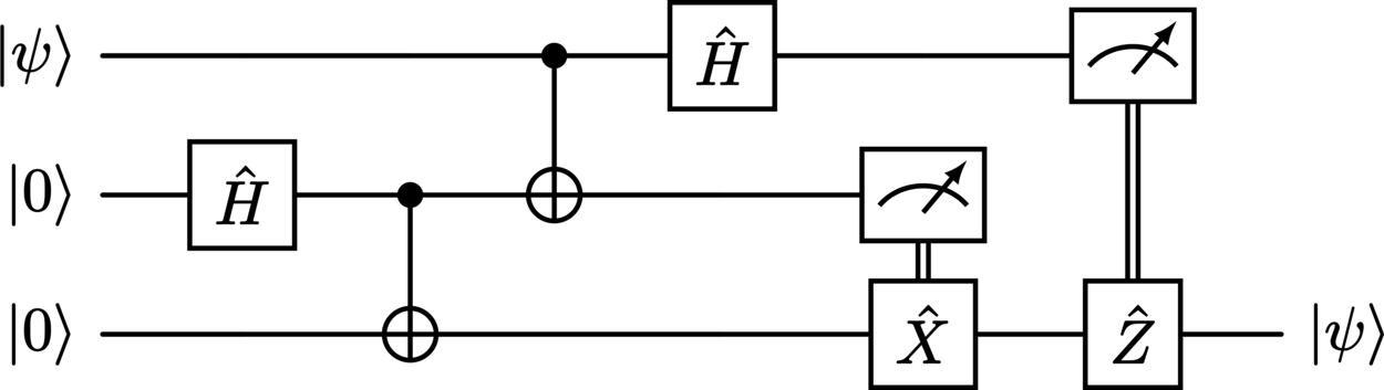
Note that in the process of teleporting the state, the original is destroyed, and so the no-cloning theorem remains unviolated. Additionally, because classical information needs to be sent between the two parties, the teleportation cannot occur faster than the speed of light, meaning that the laws of (special) relativity are satisfied. This example (Figure 26) implements the canonical version of the algorithm.

Protocol#
The canonical protocol of quantum teleportation involves three qubits divided across two parties, which are often referred to as \(A\) and \(B\) and contain two qubits and one qubit, respectively. These are initialized in the state
where \(\ket{\psi}\) is the state to be teleported. In our treatment here, we will, without loss of generality, write this state in the explicit form,
which is assumed to be normalized, e.g., \(\braket{\psi}{\psi} = \abs{a}^2 + \abs{b}^2 = 1\).
We first apply to this a Hadamard gate followed by a controlled-NOT, which entangles the last two qubits (\(A_1\) and \(B\)), forming a Bell state (\(\bigl|\Phi^+\bigr\rangle\)) on these systems,
This creates a quantum channel between the two parties, across which quantum information of the two entangled qubits is coupled (or shared).
It is at this point where a degree of physical (spatial) separation is manifested between the two parties. The “teleportation” phenomenon is then realized when the complete state of the first qubit \(\ket{\psi}\) is reconstructed (thereby destroying the original qubit) on the last system. This is achieved via the transmission of (classical) information about the state through a classical communication channel between parties \(A\) and \(B\). To accomplish this, the first two qubits are transformed by a controlled-NOT gate and a Hadamard gate, yielding the superposition
These qubits (party \(A\)) are then measured in the computational basis, and the outcomes of these measurements are used to determine the operations to be performed on \(B\). For any input state \(\ket{\psi}\), the probabilities are found to be uniform, i.e.,
and so all four of the possible outcomes (each of the form \(\ket{u} \otimes \ket{v}\)) are equiprobabilistic. Depending on the outcome, the \(B\) qubit is then transformed in a particular way:
If \(u = 1\), then a Pauli-\(Z\) gate (phase flip) is performed.
If \(v = 1\), then a Pauli-\(X\) gate (bit flip) is performed.
This corresponds to two bits of information transmitted over a classical communication channel from party \(A\) to \(B\). Table 9 summarizes this procedure.
Outcome |
Probability |
Transformation |
|---|---|---|
\(\ket{0} \otimes \ket{0}\) |
\(p_{00} = p_{0} p_{0} = \frac{1}{4}\) |
\(\Identity\) |
\(\ket{1} \otimes \ket{0}\) |
\(p_{10} = p_{1} p_{0} = \frac{1}{4}\) |
\(\PauliZ\) |
\(\ket{0} \otimes \ket{1}\) |
\(p_{01} = p_{0} p_{1} = \frac{1}{4}\) |
\(\PauliX\) |
\(\ket{1} \otimes \ket{1}\) |
\(p_{11} = p_{1} p_{1} = \frac{1}{4}\) |
\(\PauliZ \PauliX\) |
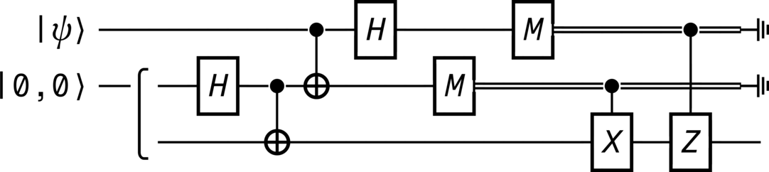
As this measurement-dependent transformation procedure concerns the exchange of purely classical information, it is depicted in the quantum circuit diagram as a pair of Pauli-\(X\) annd Pauli-\(Z\) gates with classical controls, with each classical wire connected to their respective measurement. After performing the pair of measurements and their associated transformations, the initial state on \(A_1\) is perfectly reconstructed on \(B\), which is interpreted as \(\ket{\psi}\) having “teleported” between two physically separated systems.
Implementation#
from qhronology.quantum.states import VectorState
from qhronology.quantum.gates import Hadamard, Not, Measurement, Pauli
from qhronology.quantum.circuits import QuantumCircuit
from qhronology.mechanics.matrices import ket

# Input
teleporting_state = VectorState(
    spec=[["a", "b"]],
    symbols={"a": {"complex": True}, "b": {"complex": True}},
    substitutions=[("a*conjugate(a) + b*conjugate(b)", 1)],
    label="ψ",
)
zero_state = VectorState(spec=[(1, [0, 0])], label="0,0")

# Gates
IHI = Hadamard(targets=[1], num_systems=3)
ICN = Not(targets=[2], controls=[1], num_systems=3)
CNI = Not(targets=[1], controls=[0], num_systems=3)
HII = Hadamard(targets=[0], num_systems=3)
IMI = Measurement(
    operators=[ket(0), ket(1)],
    observable=False,
    targets=[1],
    num_systems=3,
)
MII = Measurement(
    operators=[ket(0), ket(1)],
    observable=False,
    targets=[0],
    num_systems=3,
)
ICX = Pauli(index=1, targets=[2], controls=[1], num_systems=3)
CIZ = Pauli(index=3, targets=[2], controls=[0], num_systems=3)

# Circuit
teleporter = QuantumCircuit(
    inputs=[teleporting_state, zero_state],
    gates=[IHI, ICN, CNI, HII, IMI, MII, ICX, CIZ],
    traces=[0, 1],
)
teleporter.diagram(force_separation=True)

# Output
teleported_state = teleporter.state(label="ρ")

# Results
teleporting_state.print()
teleported_state.print()
print(teleporting_state.distance(teleported_state))
print(teleporting_state.fidelity(teleported_state))
Output#
Diagram#
>>> teleporter.diagram(force_separation=True)

States#
>>> teleporting_state.print()
|ψ⟩ = a|0⟩ + b|1⟩
>>> teleported_state.print()
ρ = a*conjugate(a)|0⟩⟨0| + a*conjugate(b)|0⟩⟨1| + b*conjugate(a)|1⟩⟨0| + b*conjugate(b)|1⟩⟨1|
Results#
>>> teleporting_state.distance(teleported_state)
0
>>> teleporting_state.fidelity(teleported_state)
1
References
C. H. Bennett, G. Brassard, C. Crépeau, R. Jozsa, A. Peres, and W. K. Wootters, “Teleporting an unknown quantum state via dual classical and Einstein-Podolsky-Rosen channels”, Physical Review Letters, 70(13):1895–1899, 1993. DOI: 10.1103/PhysRevLett.70.1895