Deutsch-Jozsa algorithm

Description

The Deutsch-Jozsa algorithm [1] is a deterministic quantum algorithm for solving the associated Deutsch-Jozsa problem—a black box (i.e., query) problem which is specifically designed to be easy to solve on a quantum computer and difficult to solve (deterministically) on a classical computer.

In the Deutsch-Jozsa problem, we are given a function,

(374)\[f : \{0,1\}^n \rightarrow \{0,1\},\]

with the promise that \(f\) is either constant (\(f = 0\) or \(f = 1\) for the entire input domain) or balanced (\(f = 0\) for exactly half of the input domain and \(f = 1\) for the other half). The task is to determine, through querying the function (via its manifestation as a black box computer), whether \(f\) is constant or balanced.

Classically, the Deutsch-Jozsa problem can be solved deterministically with at most \(2^{n-1} + 1\) evaluations (queries) of \(f\), where \(n\) is the number of bits. This is to say that, for a deterministic algorithm, just over half of the entire input domain must be evaluated in order to be able to arrive at a solution with no possibility of error. Alternatively, in the statistically unlikely (especially for large \(n\)) best case, if \(f\) is balanced, just two evaluations are required.

Alternatively, the quantum-mechanical Deutsch-Jozsa algorithm solves the query problem, without error, in a single evaluation of \(f\). As such, although solving the Deutsch-Jozsa problem is of little practical use, it is an example of a problem where there exists a quantum algorithm that is exponentially faster than any possible deterministic classical algorithm.

Note that the Deutsch-Jozsa algorithm generalizes earlier work by David Deutsch, specifically that of Deutsch’s algorithm [2], which is historically one of the first quantum algorithms to demonstrate a quantum advantage (i.e., a reduction in query complexity compared to the classical case). In this simplier variant, which concerns the special case of \(n=1\), the query problem is solved non-deterministically, with a probability of success of \(1/2\).

It is also important to note that, while deterministic, the first incarnation of the Deutsch-Jozsa algorithm (as it was originally presented in 1992) required exactly two queries of \(f\). Later improvements by Cleve et al. [3] resulted in an algorithm that is both deterministic and requires only a single query of \(f\), and it is this form that is known today canonically as the “Deutsch-Jozsa algorithm”.

Algorithm

In the Deutsch-Jozsa algorithm (depicted in Figure 27), querying of the function \(f\) is implemented as an oracle \(\Oracle_f\), which has the action

(375)\[\Oracle_f \ket{x} \otimes \ket{y} = \ket{x} \otimes \ket{y \oplus f(x)}.\]

Figure 27 The Deutsch-Jozsa algorithm.

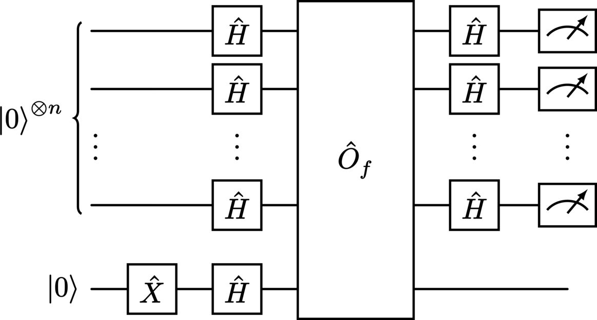
The input to the algorithm consists of two registers: the \(n\)-qubit address register and the single-qubit target register, which are initalized to the states \(\ket{0}^{\otimes n}\) and \(\ket{0}\), respectively. This gives a total input state of

(376)\[\ket{\Psi_0} = \ket{0}^{\otimes n} \otimes \ket{0}.\]

The first step of the algorithm is to transform the target qubit to a \(\ket{1}\) state, which is achieved with a Pauli-\(X\) gate on its register, i.e.,

(377)\[\begin{split}\begin{aligned} \ket{\Psi_1} &= \PauliX^{\indices{n}} \ket{\Psi_0} \\ &= (\Identity^{\otimes n} \otimes \PauliX) \ket{\Psi_0} \\ &= \ket{0}^{\otimes n} \otimes \ket{1}. \end{aligned}\end{split}\]

Next, all systems are transformed by a Hadamard gate, yielding the superposition

(378)\[\begin{split}\begin{aligned} \ket{\Psi_2} &= \Hadamard^{\otimes (n+1)} \ket{\Psi_1} \\ &= \ket{+}^{\otimes n} \otimes \ket{-} \\ &= \frac{1}{\sqrt{2^{n+1}}} \sum_{x = 0}^{2^n - 1} \ket{x} \otimes \bigl(\ket{0} - \ket{1}\bigr), \end{aligned}\end{split}\]

where each \(x\) represents a number from \(0\) to \(2^n - 1\) encoded as an \(n\)-qubit string. Applying the oracle then gives

(379)\[\begin{split}\begin{aligned} \ket{\Psi_3} &= \Oracle_f \ket{\Psi_2} \\ &= \frac{1}{\sqrt{2^{n+1}}} \sum_{x = 0}^{2^n - 1} \ket{x} \otimes \bigl(\ket{0 \oplus f(x)} - \ket{1 \oplus f(x)}\bigr) \\ &= \frac{1}{\sqrt{2^{n+1}}} \sum_{x = 0}^{2^n - 1} (-1)^{f(x)} \ket{x} \otimes \bigl(\ket{0} - \ket{1}\bigr), \end{aligned}\end{split}\]

where \(\oplus\) denotes addition (modulo \(2\)). Finally, transforming the address register with Hadamard gates results in the final output state

(380)\[\begin{split}\begin{aligned} \ket{\Psi_4} &= (\Hadamard^{\otimes n} \otimes \Identity) \ket{\Psi_3} \\ &= \frac{1}{2^{n}} \sum_{y = 0}^{2^n - 1} \sum_{x = 0}^{2^n - 1} (-1)^{f(x)} (-1)^{x \cdot y} \ket{y} \otimes \ket{-}, \end{aligned}\end{split}\]

where the used the general form of the Hadamard operator’s action

(381)\[\Hadamard^{\otimes n} \ket{k} = \frac{1}{\sqrt{2^{n}}} \sum_{j = 0}^{2^n - 1} (-1)^{j \cdot k} \ket{j}\]

with the bitwise product

(382)\[j \cdot k \equiv \bigoplus_{i = 0}^{n - 1} j_i k_i.\]

Performing a measurement on the address register in the computational basis yields the probability of obtaining an output state of \(\ket{z}\) to be

(383)\[p_z = \abs{\frac{1}{2^n} \sum_{x = 0}^{2^n - 1} (-1)^{f(x)} (-1)^{x \cdot z}}^2.\]

The probability of measuring an outcome of \(z = 0\), corresponding to \(\ket{0}^{\otimes n}\), is therefore

(384)\[\begin{split}\begin{aligned} p_0 &= \abs{\frac{1}{2^n} \sum_{x = 0}^{2^n - 1} (-1)^{f(x)}}^2 \\ &= \begin{cases} 1, & \text{if } f \text{ is constant}; \\ 0, & \text{if } f \text{ is balanced}. \end{cases} \end{aligned}\end{split}\]

The bifurcation in this result—the forking of the output into two distinct, discrete values—is due to inteference in the summation: constructive interference when \(f\) is constant and destructive interference when \(f\) is balanced. This means that, when we measure the output state to be \(\ket{0}^{\otimes n}\), the function \(f\) must be constant, while obtaining any other output state signifies that \(f\) must be balanced.

Implementation

It is useful to note that, given the action of the Deutsch-Jozsa oracle as per (375), a defintion of the oracle as an operator is simply

(385)\[\Oracle_f = \sum_{x,y = 0}^{2^n - 1} \Bigl[\bigl(1 - f(x)\bigr) \ket{x}\bra{x} \otimes \ket{y}\bra{y} + f(x) \ket{x}\bra{x} \otimes \ket{y \oplus 1}\bra{y}\Bigr].\]

This may alternatively be written equivalently as

(386)\[\Oracle_f = \bigoplus_{x = 0}^{2^n - 1} \left[\bigl(1 - f(x)\bigr) \Identity + f(x) \PauliX \right],\]

which is the definition used in the implementation here.

Code Block 31 /text/examples/algorithms/deutsch_jozsa.py

from qhronology.quantum.gates import Pauli, GateStack, Hadamard, QuantumGate
from qhronology.quantum.circuits import QuantumCircuit
from qhronology.mechanics.matrices import ket

import random
import numpy as np
from scipy.linalg import block_diag

n = 4  # The number of qubits in the address register

constant = None  # Whether the function is constant (True) or balanced (False)
constant = random.choice([True, False]) if constant is None else constant


class Oracle:
    def __init__(self, constant: bool, num_address: int):
        self.constant = constant
        self.num_address = num_address

        if self.constant is True:
            image = [random.choice([0, 1])] * 2**num_address
        else:
            image = [0] * (2**num_address // 2) + [1] * (2**num_address // 2)
        random.shuffle(image)
        self.image = image

    def f(self, x: int) -> int:
        return self.image[x]

    def operator(self) -> np.ndarray:
        blocks = [
            (1 - self.f(x)) * np.eye(2) + self.f(x) * np.eye(2)[::-1]
            for x in range(0, len(self.image))
        ]
        return np.array(block_diag(*blocks))


# Gates
IX = Pauli(index=1, targets=[n], num_systems=n + 1)
HH = GateStack(*[Hadamard()] * (n + 1))

oracle = Oracle(constant=constant, num_address=n)
O = QuantumGate(
    spec=oracle.operator(),
    targets=list(range(0, n + 1)),
    num_systems=n + 1,
    label=" O ",
)

HI = GateStack(*[Hadamard()] * n)

# Circuit
deutsch_jozsa = QuantumCircuit(
    gates=[IX, HH, O, HI],
    numerical=True,
    array=True,
)
deutsch_jozsa.diagram(pad=(1, 0), sep=(1, 2), force_separation=True)

# Measurement
probabilities = deutsch_jozsa.measure(
    operators=[ket([0] * n)],
    targets=list(range(0, n)),
    observable=False,
    statistics=True,
)
probability_zeroes = np.round(np.real(probabilities[0])).astype(int)

result_constant = True if probability_zeroes == 1 else False
result_function = "constant" if oracle.constant is True else "balanced"
result_algorithm = "constant" if result_constant is True else "balanced"

# Results
print(f"The function: {result_function}")
print(f"The Deutsch-Jozsa result: {result_algorithm}")

Output

Diagram

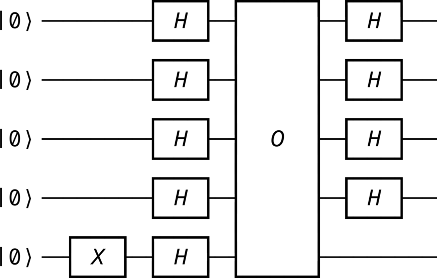
>>> deutsch_jozsa.diagram(pad=(1, 0), sep=(1, 2), force_separation=True)

Results

If constant is True:

>>> print(f"The function: {result_function}")
The function: constant

>>> print(f"The Deutsch-Jozsa result: {result_algorithm}")
The Deutsch-Jozsa result: constant

If constant is False:

>>> print(f"The function: {result_function}")
The function: balanced

>>> print(f"The Deutsch-Jozsa result: {result_algorithm}")
The Deutsch-Jozsa result: balanced

References

[1]

D. Deutsch and R. Jozsa, “Rapid solution of problems by quantum computation”, Proceedings of the Royal Society of London. Series A: Mathematical and Physical Sciences, 439(1907):553–558, December 1992. DOI: 10.1098/rspa.1992.0167

[2]

D. Deutsch, “Quantum theory, the Church–Turing principle and the universal quantum computer”, Proceedings of the Royal Society of London. A. Mathematical and Physical Sciences, 400(1818):97–117, July 1985. DOI: 10.1098/rspa.1985.0070

[3]

R. Cleve, A. Ekert, C. Macchiavello, and M. Mosca, “Quantum algorithms revisited”, Proceedings of the Royal Society A: Mathematical, Physical and Engineering Sciences, 454(1969):339–354, January 1998. DOI: 10.1098/rspa.1998.0164