


Shor’s factorization algorithm#
Description#
Shor’s factorization algorithm [1, 2], often called just Shor’s algorithm, is an innovative quantum algorithm for the factorization of integers. An instance of the hidden subgroup problem, the algorithm’s significance lies in its ability to factor large integers in polynomial time, which is exponentially faster than any known classical algorithm.
Shor’s algorithm is a notable example of a hybrid algorithm, in which both classical and quantum processing are employed in order to obtain the desired outcome. As part of the algorithm, the factorization problem is reduced down to the problem of order-finding, a process known as classical reduction. Solving the order-finding problem then forms the core of the algorithm, and is the only component which is performed quantum mechanically (via quantum phase estimation—see eg:phase_estimation Quantum phase estimation).
Integer factorization#
Formally, the factorization of an arbitrary positive integer \(N\) involves determining a pair of positive integers \(p, q\) such that
If either of \(p\) and \(q\) is composite, then factorization of the factor itself can occur. Repeatedly decomposing all factors in this manner eventually results in a sequence of prime numbers \((n_k)_k\) where their product reconstructs \(N\), e.g.,
This process is known as prime factorization, and by the prime factorization theorem, the sequence of prime factors \((n_k)_k\) is always unique (up to its order).
Formulating an algorithm to perform factorization on a classical computer is not unobtainable, with a plethora of such algorithms already existing, including Euclid’s algorithm. However, formulating a factorization algorithm that is sufficiently efficient for large integers is currently an open problem: no classical algorithm which can perform integer factorization in polynomial time (i.e., a time complexity of \(\BigO(n^k)\) for input of size \(n\) and some positive constant \(k\)) have been found to date. Fortunately, Shor’s algorithm presents a quantum approach for efficient integer factorization, with significant applications in fields such as cryptography and computational mathematics.
The order-finding problem#
Given the set of integers \(\Integers\), we can, using a positive integer \(N \in \IntegersPositive\), define a subset as
If we only include elements in this set which are coprime to \(N,\) (which necessarily satisfy \(\gcd(N, n) = 1\)), then we obtain
Under the operation of (modular) multiplication, this set forms a group, and is sometimes written as \((\Integers \setminus n\Integers)^\times\) (and variations thereof).
Note
Suppose \(G_m\) is a modulo multiplication group with the group operation of multiplication (modulo \(m\)), and let \(1_G \in G_m\) denote its multiplicative identity. If \(g \in G_m\) is an element of the group, then there exists a positive integer \(\abs{G}\) such that \(g^{\abs{G}} = 1_G \; (\mathrm{mod} \; m)\). Here, \(\abs{G}\) is called the order of \(G_m\), and \(g^{\abs{G}}\) denotes the multiplication of \(g\) by itself exactly \(\abs{G}\) times.
As \(\Integers_N^*\) is the multiplicative group of integers modulo \(N\), then we can repeatedly multiply any element \(a \in \Integers_N^*\) by itself and eventually obtain \(1\). Mathematically, this means that for each base \(a\) there exists a finite number of modular multiplications \(r\) such that
Note that the value of \(r\) is specific to that combination of both the element \(a\) and the modulus \(N\).
Of course, if \(r\) satisfies (412), then so will any exponent of the form \(r + k\), where \(k\) is a positive integer. The smallest possible non-zero value of \(r\) for which this holds true is called the order of the element \(a\). This can be expressed more eloquently; by defining the modular exponential function,
we can write
Due to its modularity, \(f\) is periodic, with \(r\) serving as its period, i.e.,
for any positive integer \(k\). Determining the smallest possible value(s) of \(r\) for which any given (univariate) function \(f\) is periodic, e.g., \(f(x + r) = f(x)\) (for all \(x\)), constitutes the problem of period-finding. In the special case of the modular exponent function (413), determining such an integer \(r\) such that (414) holds true (given positive integers \(N\) and \(a\), with \(\gcd(N, a) = 1\)) is called order-finding.
Factorization by order-finding#
Solving the problem of order-finding is useful because it can be used to factorize an integer. This is achieved by first assigning the number to be factorized \(N\) as the modulus of the associated multiplicative group of integers. The period \(r\) is then calculated given an element \(a \in \Integers_N^* \setminus \{1\}\) (so \(N\) and \(a\) are coprime). Since (412) is satisfied for such values of \(a\), then \(N\) divides \(a^{r} - 1\), which is often written as
This simply means that there exists an integer \(z\) such that \(a^{r} - 1 = zN\). By factorizing this expression algebraically, we obtain the product
If \(r\) is odd, then the period should be recomputed using a different value for \(a\). When \(r\) is determined to be even, then \(r/2\) is an integer, and so \(a^{r/2}\) is the non-trivial square root of \(a^{r}\). Proceeding under this assumption, we have
which may imply the following two statements:
Neither of these statements can be true if the factorization algorithm is to be successful. If (i) holds, then we must have \(a^{r/2} = 1 \; (\mathrm{mod} \; N)\). However, this contradicts the fact that \(r\) is the order of \(a\), and so (i) is always false (provided a correct \(r\) was found). Thus, (i) cannot be true. We subsequently compute the value
If \(d = 1\), then statement (ii) is true, and the factorization procedure has trivial factor (either \(1\) or \(N\)) and should be repeated with a different value for \(a\) (to attempt to find a non-trivial factor). Alternatively, if \(d > 1\), then
are non-trivial factors of \(N\), e.g., \(N = pq\), with neither value being equal to \(1\) or \(N\).
Algorithm#
Before executing Shor’s algorithm for a given number \(N\), it can be advantageous to perform a few (purely classical) pre-processing checks in order to maximize efficiency. In particular, the complexity of the problem can be greatly reduced for certain classes of integers. First are the even numbers: using Euclid’s algorithm, we can efficiently compute the greatest common divisor (GCD) between two integers, meaning that we can check whether \(N\) is even (in which case 2 is trivially a factor). Then, we can also check whether \(N\) is a prime power, for which efficient classical factorization algorithms already exist (and so we need not perform Shor’s algorithm). The version of Shor’s algorithm presented here therefore assumes that the number \(N\) to be factorized is neither even or a prime power.
Choose, at random, an integer \(a \in \Integers_N \setminus \{1\}\).
Classical pre-processing: Compute \(d = \gcd(N, a)\).
If \(d > 1\), then factors have been found: output \(p = d\) and \(q = N/d\). Exit.
If \(d = 1\), then \(a\) and \(N\) are coprime (therefore \(a \in \Integers_N^*\)). Continue.
Quantum order-finding: Find the period \(r\) such that \(a^r \; \mathrm{mod} \; N = 1\).
Classical post-processing:
If \(r\) is even, then compute \(a^\prime = a^{r/2} - 1 \; \mathrm{mod} \; N\) and \(d^\prime = \gcd(N, a^\prime)\).
If \(d^\prime > 1\), then factors have been found: output \(p = d^\prime\) and \(q = N/d^\prime\). Exit.
If \(d^\prime = 1\), then the algorithm has failed to factorize \(N\). Goto step 1.
If \(r\) is odd, then the algorithm has failed to factorize \(N\). Goto step 1.
This is, in essence, a complete description of Shor’s algorithm, with the understanding that the order-finding step is performed efficiently via a phase estimation subroutine on a quantum computer (see eg:shor_estimation Order-finding via quantum phase estimation).
Evidently, as a probabilistic algorithm, there is a chance that it can fail on any given run. This happens in two specific situations:
The computed period \(r\) is odd.
The computed period \(r\) is even and \(\gcd(N, a^{r/2} - 1) = 1\).
For a random choice of \(a\), the probability of either of the two failing events occuring is at most \(2^{-(s-1)}\), where \(s\) is the number of distinct prime factors of \(N\). The probability of any given run being successful is therefore at least \(0.5\), and so executing the algorithm \(t\) times (each with a randomly chosen \(a\)) results in a probability of success being bounded from below by \(1 - 2^{-t}\). Much of the trial-and-error associated with the algorithm’s probabilistic nature can therefore be eliminated by providing \(a\) such that it is coprime to \(N\) (i.e., \(a \in \Integers_N^*\)), in cases where such knowledge is possible.
Order-finding via quantum phase estimation#
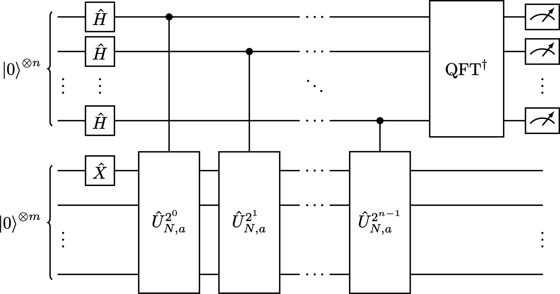
Quantum phase estimation (see eg:phase_estimation Quantum phase estimation) presents an efficient method of order-finding that is unattainable through classical means. This is achieved through using operators that have the action
as the base of the controlled-\(\Unitary\) gates in the phase estimation algorithm. Note that, given this definition, it is easy to verify that
and so, in the case of \(z = 1\), we have
The phase estimation procedure then simply determines the smallest integer value of \(r\) (i.e., the period) for which
thereby solving the order-finding problem. This is achieved by using the decoded phase value \(\theta\), obtained from the phase estimation itself, to calculate the integer \(r\) via the relation \(\theta = 1/r\). The quantum circuit depicting the phase estimation procedure in Shor’s algorithm appears in Figure 29.

Implementation#
The implementation of Shor’s algorithm presented here diverges from typical implementations in two significant ways:
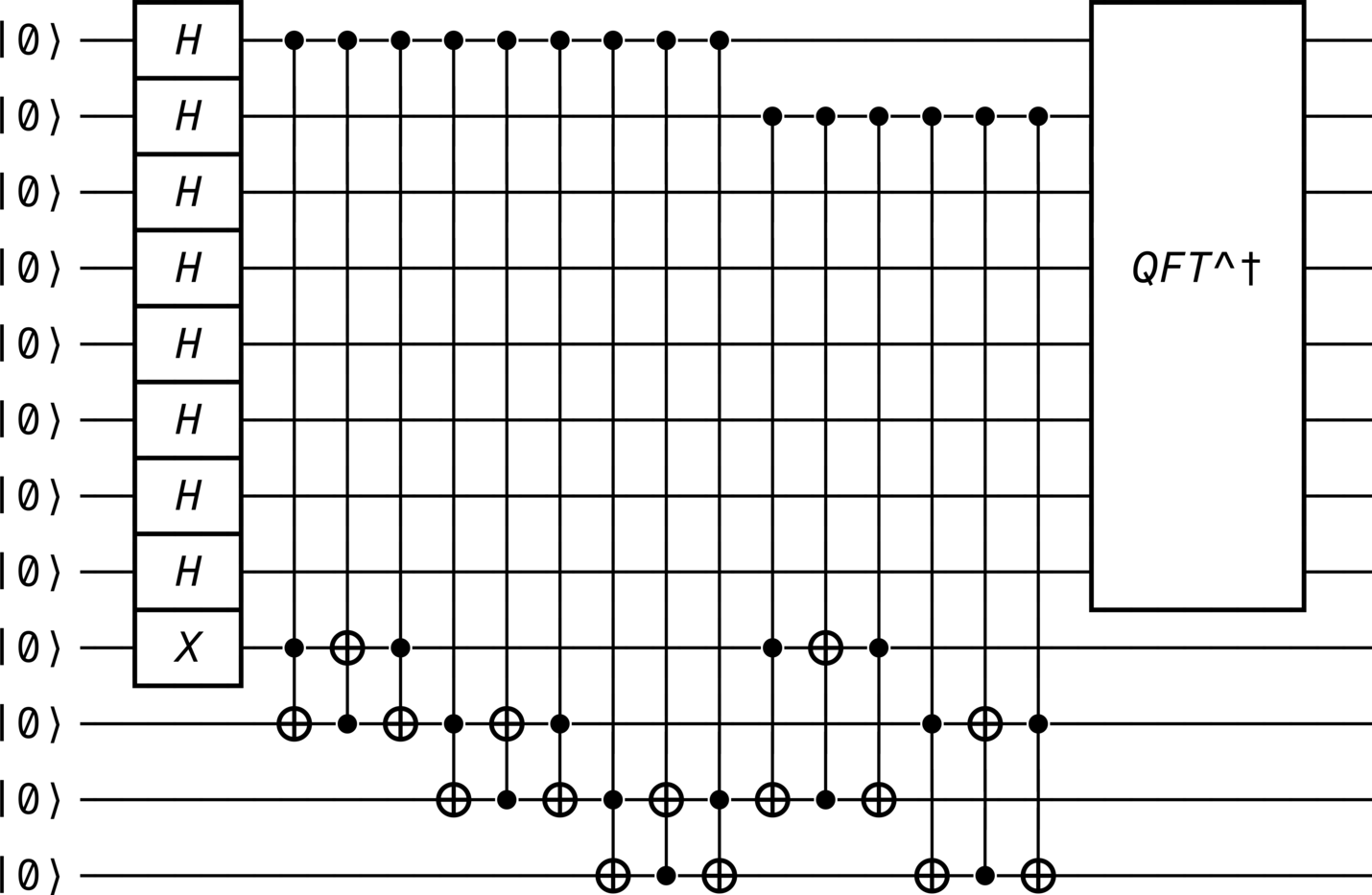
The modular exponentiation gates are constructed artificially, by generating their corresponding operators’ matrix representations from first principles. Decompositions of these gates in terms of CNOTs can then be computed and subsequently employed, depending on the value of the
decompose(bool) variable.Instead of repeating the simulation numerous times to obtain a probability distribution of outcomes, we extract the exact probabilities themselves directly via measurement after a single simulation, and use them to determine the (likely) factors. This is far more computationally efficient, though the circuit can be easily adapted if a more faithful recreation of experiment is desired.
Note that in this implementation of Shor’s algorithm, the two registers of the quantum phase estimation procedure employ \(2n\) and \(n\) qubits, respectively, where \(n\) is the minimum number of qubits required to encode the number \(N\). Analysis shows that \(2n\) qubits in the estimation (upper) register is the minimum number that is able to provide the precision necessary in order to correctly distinguish between different periods in every case. However, particularly for small \(N\), the algorithm can often be successfully executed using just \(n\) estimation qubits. It is also useful to be aware that versions of the algorithm in the literature often employ certain optimizations with which they can use fewer qubits to achieve the same result.
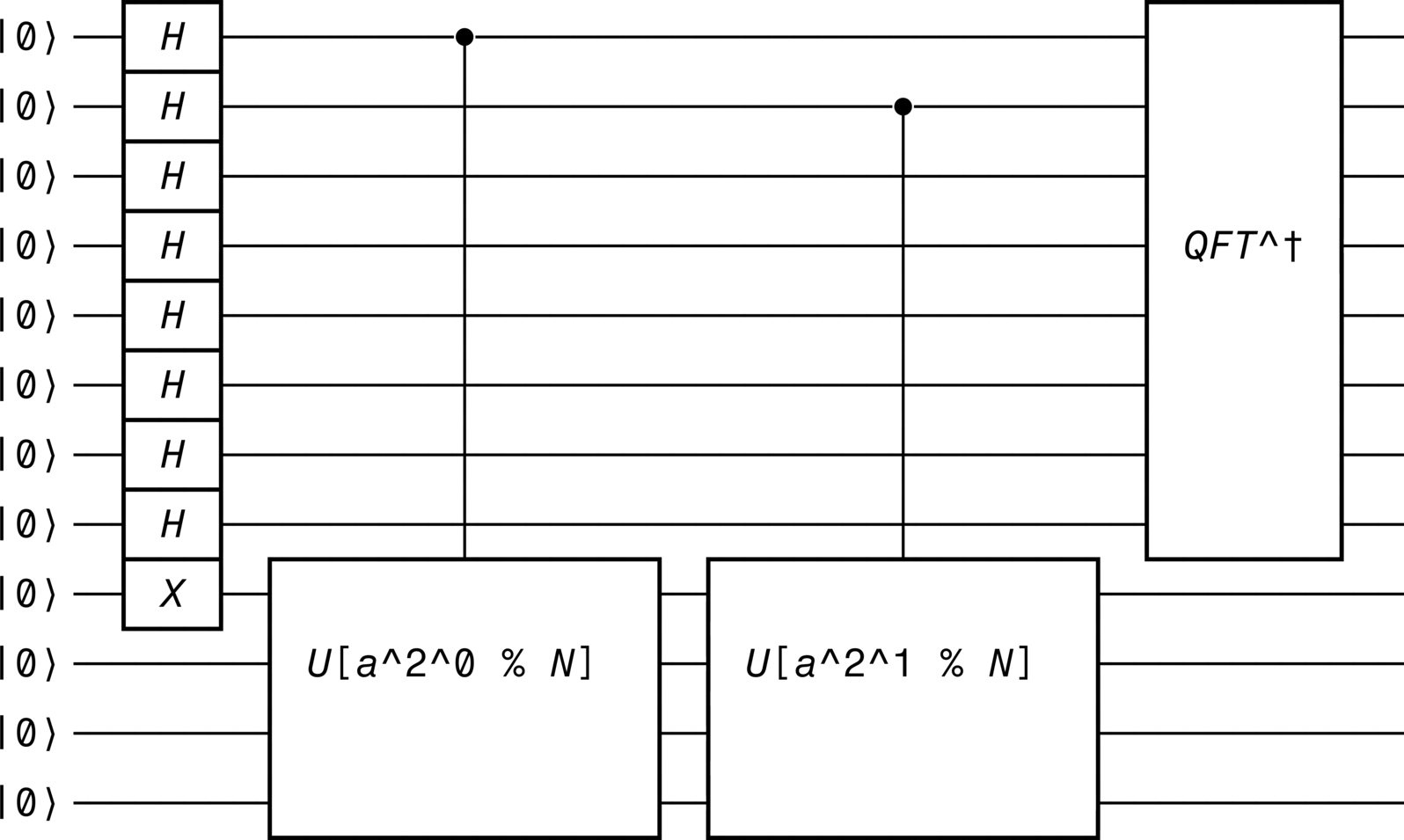
As evident by the simulation’s results that appear below, the number of controlled-\(\Unitary\) gates need not always be equal to the number of systems in the estimation register. This is because there can be instances (values of \(j\) given \(N\) and \(a\)) where the modular exponentiation gate \(\Unitary_{N,a}^{2^j}\) is equivalent to the identity gate \(\Identity\), and so application of the corresponding controlled-\(\Unitary\) gate is redundant.
It is also worth mentioning that while this implementation supports any valid (factorizable) positive integer \(N\) as input (set with the variable N), attempting to factorize those larger than 15 (corresponding to more than 12 qubits in total across both registers) can require significant amounts of both memory and time.
from qhronology.quantum.gates import GateStack, Hadamard, Pauli, QuantumGate, Fourier, Swap, Not
from qhronology.quantum.circuits import QuantumCircuit
from qhronology.mechanics.matrices import encode, decode
from qhronology.mechanics.operations import dagger

import math
from fractions import Fraction
import sympy as sp
import numpy as np

N = 15  # The number to be factorized
a = 2  # Should be coprime to N
decompose = False  # Whether to decompose the modular exponentiation

n = int(math.ceil(math.log(N + 1, 2)))  # Encoding depth

num_controls = 2 * n
num_targets = n
num_total = num_targets + num_controls

systems_controls = list(range(0, num_controls))
systems_targets = [k + num_controls for k in range(0, num_targets)]

# Gates
HX = GateStack(
    *[Hadamard()] * num_controls,
    Pauli(index=1),
)


# Function for computing modular exponentiation
def mod_exp_function(base: int, power: int, modulus: int) -> int:
    """Compute a^{2^j} (mod N)."""
    value = base
    for _ in range(power):
        value = int(value**2 % modulus)
    return value


# Function for constructing modular exponentiation operators
def mod_exp_operator(
    base: int,
    power: int,
    modulus: int,
    num_systems: int | None = None
) -> np.ndarray:
    """Compute U_{N,a}^{2^j}."""
    value = mod_exp_function(base, power, modulus)
    num_systems = (
        int(math.ceil(math.log(modulus + 1, 2)))
        if num_systems is None else num_systems
    )

    untransformed = list(range(0, 2**num_systems))
    transformed = [
        (value * k) % (2**num_systems - 1) for k in untransformed
    ]

    operator = np.zeros((2**num_systems, 2**num_systems), dtype=complex)
    for pair in zip(untransformed, transformed):
        operator += encode(
            pair[1], num_systems, numerical=True, array=True
        ) * dagger(encode(
            pair[0], num_systems, numerical=True, array=True
        ))
    operator[(0, -1)] = 0
    operator[(-1, -1)] = 1
    return operator


# Construct modular exponentiation gates
mod_exp_gates = []
for j in systems_controls:
    operator = mod_exp_operator(a, j, N)
    if (
        mod_exp_function(a, j, N) != 1
        or np.array_equal(operator, np.eye(2**n, dtype=complex)) is False
    ):
        mod_exp_gates.append(
            QuantumGate(
                spec=operator,
                targets=systems_targets,
                controls=[systems_controls[j]],
                num_systems=num_total,
                label=f"U[a^2^{j} % N]",
                numerical=True,
                array=True,
            )
        )

# Decompose modular exponentiation gates
# (Note: this is not possible for every combination of N and a)
if decompose is True:
    # Decompose into SWAP gates
    for g, gate in enumerate(mod_exp_gates):
        mod_exp_gates[g] = gate.decompose(
            gates=[Swap()],
            depth=n,
        )[0]
    mod_exp_gates = [
        gate for sequence in mod_exp_gates
        for gate in sequence
    ]
    # Decompose into CNOT gates
    for g, gate in enumerate(mod_exp_gates):
        mod_exp_gates[g] = gate.decompose(
            gates=[Not()],
            additional_nodes=(0, 1, 0),
        )[0]
    mod_exp_gates = [
        gate for sequence in mod_exp_gates
        for gate in sequence
    ]

IQFT = Fourier(
    targets=systems_controls,
    num_systems=num_total,
    composite=True,
    conjugation=True,
    label="QFT^†",
)

# Circuit
shor = QuantumCircuit(
    gates=[HX] + mod_exp_gates + [IQFT],
    numerical=True,
    array=True,
)
shor.diagram(pad=(1, 0), force_separation=True)

# Measurement
basis = [encode(k, num_controls) for k in range(0, 2**num_controls)]
probabilities = shor.measure(
    operators=basis,
    targets=systems_controls,
    observable=False,
    statistics=True,
)
probabilities = [np.real(probability) for probability in probabilities]

# Results
print(f"Input number: {N}")
threshold = 0.01
for k, probability in enumerate(probabilities):
    if probability >= threshold or probability == max(probabilities):
        probability = sp.N(probability).round(3)
        phase = decode(basis[k]) / 2**num_controls
        r = Fraction(phase).limit_denominator(N - 1).denominator
        bitstring = encode(
            decode(basis[k], reverse=True),
            num_controls,
            return_type=str,
        )

        suffix = "(period not suitable)"
        if r % 2 == 0:
            p = math.gcd(a ** int(r / 2) - 1, N)
            q = math.gcd(a ** int(r / 2) + 1, N)

            if not p * q == N:
                p, q = p * q, int(N / (p * q))
            if p * q == N and p > 1 and q > 1:
                suffix = f"Factors: {p} and {q}"
            else:
                suffix = "(algorithm failed)"

        print(
            f"Bitstring={bitstring}, "
            + f"Probability={probability}, "
            + f"Period={r}, "
            + f"{suffix}"
        )
Output#
Diagram#
If decompose is False:
>>> shor.diagram(pad=(1, 0), force_separation=True)

If decompose is True:
>>> shor.diagram(pad=(1, 0), force_separation=True)

Results#
Cumulative output from the various print statements:
Input number: 15
Bitstring=00000000, Probability=0.250, Period=1, (period not suitable)
Bitstring=00000010, Probability=0.250, Period=4, Factors: 3 and 5
Bitstring=00000001, Probability=0.250, Period=2, Factors: 3 and 5
Bitstring=00000011, Probability=0.250, Period=4, Factors: 3 and 5
References
P. W. Shor, “Algorithms for quantum computation: discrete logarithms and factoring”, Proceedings 35th Annual Symposium on Foundations of Computer Science, pages 124–134, November 1994. DOI: 10.1109/SFCS.1994.365700
P. W. Shor, “Polynomial-Time Algorithms for Prime Factorization and Discrete Logarithms on a Quantum Computer”, SIAM Journal on Computing, 26(5):1484–1509, October 1997. DOI: 10.1137/S0097539795293172