Fourier transform decomposition

Description

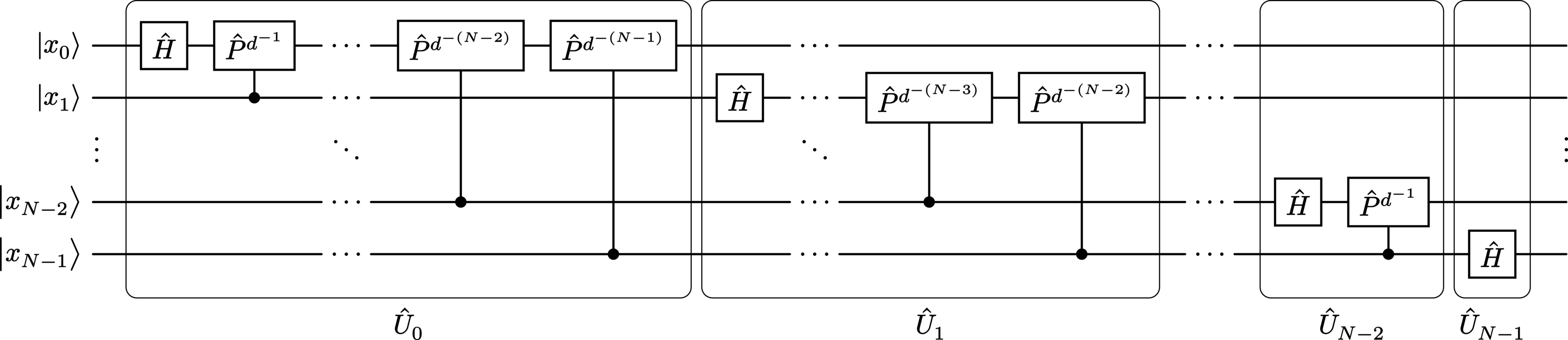
A canonical decomposition of the multipartite (composite) quantum Fourier transform \(\QFT_N\) (over \(N\)-qudits) consists of a succession of sequences of Hadamard and phase gates. Depicted in Figure 16, this can be written mathematically as

(346)\[\QFT_N = \prod_{n = 0}^{N - 1} \Unitary_n\]

where

(347)\[\Unitary_n = \left(\prod_{j = 1}^{N - 1 - n} \Control^{\indices{n + j}} \bigl(\Phase^{d^{-j}}\bigr)^{\indices{n}} \right) \cdot \Hadamard^{\indices{n}}.\]

Here,

(348)\[\Phase = \sum_{k=0}^{d-1} \omega^{k} \ket{k}\bra{k}\]

is the \(d\)-dimensional phase gate with \(\omega \equiv \e^{2\pi\eye/d}\).

Figure 16 A decomposition of the quantum Fourier transform.

Implementation

Code Block 21 /text/examples/algorithms/fourier_transform.py

from qhronology.quantum.gates import Hadamard, Phase
from qhronology.quantum.circuits import QuantumCircuit

import sympy as sp

size = 4  # The number of qudits
dim = 2  # The dimensionality of the Fourier transform

# Gates
QFT = []
for i in range(0, size):
    count = size - i
    for j in range(0, count):
        if j == 0:
            QFT.append(
                Hadamard(
                    targets=[i],
                    num_systems=size,
                    dim=dim,
                )
            )
        else:
            QFT.append(
                Phase(
                    targets=[i],
                    controls=[i + j],
                    exponent=sp.Rational(1, dim**j),
                    num_systems=size,
                    dim=dim,
                    label=f"{dim**j}",
                    family="GATE",
                )
            )

# Circuit
fourier = QuantumCircuit(gates=QFT)
fourier.diagram(sep=(0, 1), visible={"gates"})

# Results
print(repr(fourier.gate()))

Output

Note that the total operator’s matrix representation is far too large to display here.

Diagram

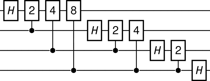
>>> fourier.diagram(sep=(0, 1), visible={"gates"})

References