Quantum phase estimation

Description

If \(\lambda\) is an eigenvalue of a given unitary operator \(\Unitary\) corresponding to a given eigenvector \(\ket{\psi}\), then we have

(387)\[\Unitary\ket{\psi} = \lambda\ket{\psi}.\]

Since unitary operators represent transformations around the unit circle, then their eigenvalues necessarily have unit modulus, i.e., \(\abs{\lambda} = 1\). This means that any such eigenvalue can be written in the form

(388)\[\lambda = \e^{2\pi\eye\theta},\]

and so is characterized completely by its phase \(\theta \in \Reals\). Note that, due to the peridocity of the complex exponential, this may be taken on the restricted domain \(0 \leq \theta < 1\). Quantum phase estimation is then simply a procedure for estimating this phase \(\theta\) given both a unitary operator \(\Unitary\) and an eigenvector \(\ket{\psi}\).

Algorithm

In the canonical quantum phase estimation algorithm, introduced by Kitaev [1] and depicted in Figure 28, we require two registers. The first (upper), called the estimation (or control) register, consists of \(n\) qubits (on the Hilbert space \(\SpaceHilbert_2^{\otimes n}\)), with each initialized to \(\ket{0}\). The second (lower), called the eigenvector (or target) register, is in the state of an eigenvector \(\ket{\psi}\) of the given \(\Unitary\) over \(m\) qubits (on the Hilbert space \(\SpaceHilbert_2^{\otimes m}\)). The total initial state may therefore be written as

(389)\[\ket{\Psi_0} = \ket{0}^{\otimes n} \otimes \ket{\psi}.\]

The first step consists of transforming the estimation register to an equal superposition state. This is achieved via an \(n\)-qubit Hadamard gate operation \(\Hadamard^{\otimes n}\), which gives

(390)\[\begin{split}\begin{aligned} \ket{\Psi_1} &= (\Hadamard^{\otimes n} \otimes \Identity^{\otimes m})\ket{\Psi_0} \\ &= \ket{+}^{\otimes n} \otimes \ket{\psi} \\ &= \frac{1}{2^{n/2}}\sum_{x=0}^{2^n - 1} \ket{x} \otimes \ket{\psi}. \end{aligned}\end{split}\]

Here, \(\ket{x}\) is an \(n\)-ary representation of states in the \(n\)-qubit register, e.g.,

(391)\[\ket{x} = \bigotimes_{\ell = 0}^{n - 1} \ket{x_\ell},\]

where the binary decomposition of \(x\) is simply

(392)\[x = \sum_{\ell = 0}^{n - 1} x_\ell 2^\ell.\]

Figure 28 A quantum phase estimation algorithm.

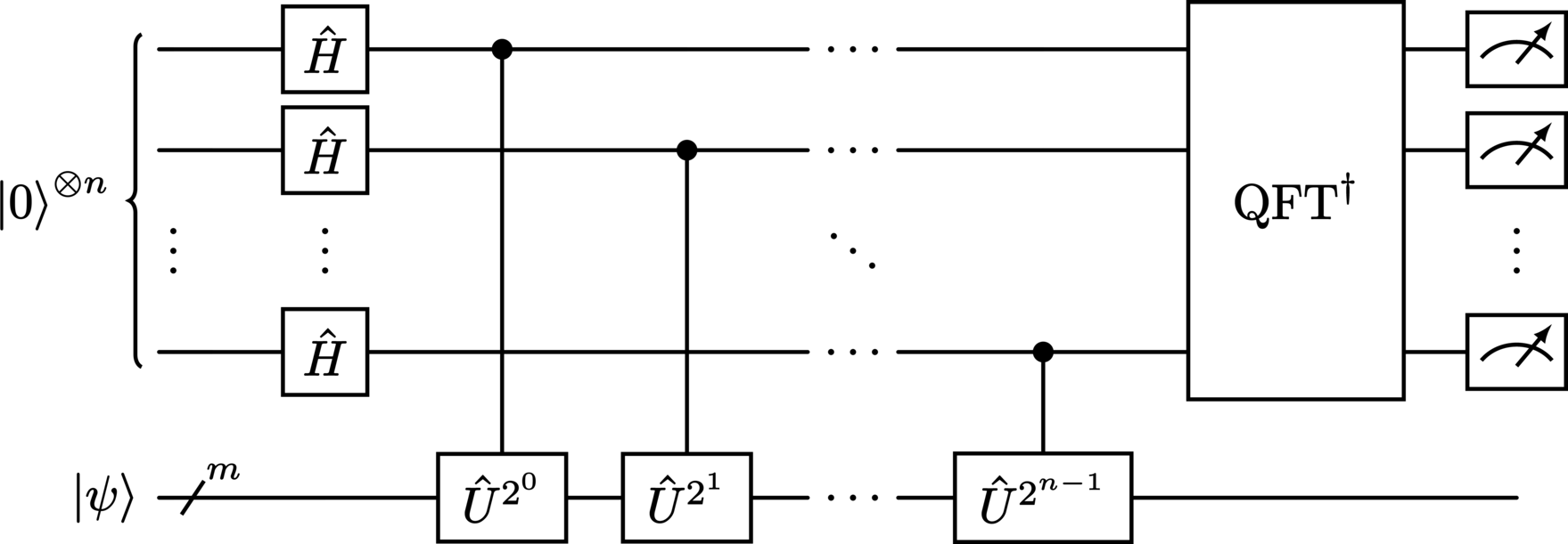
A sequence of controlled-\(\Unitary\) operations, each of the form,

(393)\[\Control^{\indices{\ell}} \Unitary^{2^\ell} = \sum_{k=0}^{1} {\ket{k}\bra{k}}^{\indices{\ell}} \otimes \bigl(\Unitary^{2^\ell}\bigr)^k\]

is then applied, where \(\ell\) is the index of the system in the estimation register. The total transformation incurred by this sequence may be written as

(394)\[\Unitary_\Control = \prod_{\ell = 0}^{n - 1} \Control^{\indices{\ell}} \Unitary = \sum_{k=0}^{2^n - 1} \ket{k}\bra{k} \otimes \Unitary^k,\]

under which the circuit’s state becomes

(395)\[\begin{split}\begin{aligned} \ket{\Psi_2} &= \Unitary_\Control \ket{\Psi_1} \\ &= \frac{1}{\sqrt{2^n}} \sum_{k=0}^{2^n - 1} \e^{2\pi\eye\theta k} \ket{k} \otimes \ket{\psi}. \end{aligned}\end{split}\]

Note that here we introduced the eigenvalue of \(\Unitary\) as \(\lambda = \e^{2\pi\eye\theta}\) (corresponding to the eigenvector \(\ket{\psi}\)), and subsequently used the fact that

(396)\[\Unitary^{k} \ket{\psi} = \e^{2\pi\eye\theta k} \ket{\psi}.\]

Performing an \(n\)-qubit inverse Fourier transform \(\QFT_n^\dagger\),

(397)\[\ket{k} \stackrel{\QFT_n^\dagger}{\longrightarrow} \frac{1}{\sqrt{2^n}} \sum\limits_{x=0}^{2^n - 1} \e^{-2\pi\eye k x 2^{-n}} \ket{x},\]

on the estimation register then yields the output state

(398)\[\begin{split}\begin{aligned} \ket{\Psi_3} &= (\QFT_n^\dagger \otimes \Identity) \ket{\Psi_2} \\ &= \frac{1}{\sqrt{2^n}} \sum_{k=0}^{2^n - 1} \e^{2\pi\eye\theta k} \left(\frac{1}{\sqrt{2^n}} \sum\limits_{x=0}^{2^n - 1} \e^{-2\pi\eye k x 2^{-n}} \ket{x}\right) \otimes \ket{\psi} \\ &= \frac{1}{2^{n}} \sum_{k=0}^{2^n - 1} \sum\limits_{x=0}^{2^n - 1} \e^{2\pi\eye k (\theta - x 2^{-n})} \ket{x} \otimes \ket{\psi}. \end{aligned}\end{split}\]

By inspection, the amplitude associated with each \(\ket{x}\) simply takes the form

(399)\[c_x = \frac{1}{2^{n}} \sum_{k = 0}^{2^n - 1} \e^{2\pi\eye k (\theta - x 2^{-n})},\]

and so performing a measurement in the computational basis on the estimation register yields the outcome \(\ket{y}\) with probability

(400)\[p_y = |c_y|^2 = \frac{1}{2^{2n}} \abs{\sum_{k = 0}^{2^n - 1} \e^{2\pi\eye k (\theta - y 2^{-n})}}^2.\]

With foresight, we can define the substitution

(401)\[\theta = \frac{z}{2^{n}} + \delta\]

where \(z/2^{n}\) is the nearest integer to \(\theta\), and the discrepancy \(\delta\) satisfies \(0 \leq \abs{\delta} \leq 1/2\). In effect, this approximates \(\theta \in [0, 1]\) by rounding its value to the nearest integer. With this, the probabilities take the form

(402)\[p_y = \frac{1}{2^{2n}} \abs{\sum_{k = 0}^{2^n - 1} \e^{\frac{2\pi\eye k}{2^n} (z - y)} \e^{2\pi\eye k \delta}}^2.\]

If \(\delta = 0\), the corresponding probability to find such a value \(z\) is

(403)\[p_z = \frac{1}{2^{2n}} \abs{\sum_{k = 0}^{2^n - 1} 1}^2 = 1.\]

Evidently, in such a case, the outcome is always found to be \(y = z\), and so the phase can decoded as \(\theta = z / 2^n\). Alternatively, if \(\delta \neq 0\), then the probability to find \(z\) is

(404)\[\begin{split}\begin{aligned} p_z &= \frac{1}{2^{2n}} \abs{\sum_{k = 0}^{2^n - 1} \e^{2\pi\eye k \delta}}^2 \\ &= \frac{1}{2^{2n}} \abs{\frac{1 - \e^{2\pi\eye 2^n \delta}}{1 - \e^{2\pi\eye \delta}}}^2, \end{aligned}\end{split}\]

where we used the identity

(405)\[\sum_{n = 0}^{N - 1} a^n = \frac{1 - a^N}{1 - a}, \quad a \neq 1.\]

With a little effort, it can be shown that

(406)\[p_z \geq \frac{4}{\pi^2} \approx 0.405\]

for any \(\delta \neq 0\), from which we can conclude that the algorithm provides an estimate of \(\theta\) (to within \(1/2^n\) of the actual value) with a probability of at least \(4/\pi^2\).

Implementation

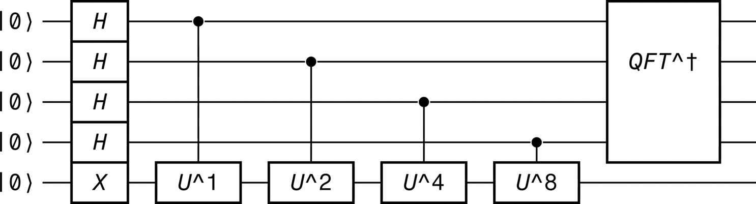
In this implementation, the target register consists of a single qubit \(\ket{\psi} = \ket{1}\), with which the unitary operator is the phase gate, specifically,

(407)\[\Unitary(\theta) = \ket{0}\bra{0} + \e^{2\pi\eye\theta} \ket{1}\bra{1}.\]

Code Block 32 /text/examples/algorithms/phase_estimation.py

from qhronology.quantum.gates import GateStack, Hadamard, Pauli, Phase, Fourier
from qhronology.quantum.circuits import QuantumCircuit
from qhronology.mechanics.matrices import encode, decode

import sympy as sp
import numpy as np

phase = 0.64  # The phase to be estimated
precision = 4  # The number of qubits used by the estimation

num_controls = precision
num_targets = 1
num_total = num_targets + num_controls

systems_controls = list(range(0, num_controls))
systems_targets = [m + num_controls for m in range(0, num_targets)]

# Gates
HX = GateStack(
    *[Hadamard()] * num_controls,
    Pauli(index=1),
)

unitaries = [
    Phase(
        phase=sp.exp(2 * sp.I * sp.pi * phase * 2**n),
        targets=systems_targets,
        controls=[systems_controls[n]],
        num_systems=num_total,
        label=f"U^{2**n}",
    )
    for n in range(0, num_controls)
]

IQFT = Fourier(
    targets=systems_controls,
    num_systems=num_total,
    composite=True,
    conjugation=True,
    label="QFT^†",
)

# Circuit
phase_estimator = QuantumCircuit(
    gates=[HX] + unitaries + [IQFT],
    numerical=True,
    array=True,
)
phase_estimator.diagram(pad=(1, 0), force_separation=True)

# Measurement
basis = [encode(k, num_controls) for k in range(0, 2**num_controls)]
probabilities = phase_estimator.measure(
    operators=basis,
    targets=systems_controls,
    observable=False,
    statistics=True,
)
probabilities = [np.real(probability) for probability in probabilities]

# Results
print(f"Input phase: {phase}")
expectation = 0
threshold = 0.001
for k, probability in enumerate(probabilities):
    value = decode(basis[k]) / 2**num_controls
    value = sp.N(value).round(precision)
    bitstring = encode(decode(basis[k]), num_controls, return_type=str)
    expectation += probability * value

    suffix = ""
    if probability == max(probabilities):
        suffix = " (most probable)"

    if probability >= threshold or probability == max(probabilities):
        probability = sp.N(probability).round(3)
        print(
            f"Bitstring={bitstring}, "
            + f"Probability={probability}, "
            + f"Phase={value}"
            + f"{suffix}"
        )

expectation = sp.N(expectation).round(precision)
print(f"Expectation (weighted average): {expectation}")

Output

Diagram

>>> phase_estimator.diagram(pad=(1, 0), force_separation=True)

Results

Cumulative output from the various print statements:

Input phase: 0.64
Bitstring=0000, Probability=0.002, Phase=0
Bitstring=0001, Probability=0.002, Phase=0.0625
Bitstring=0010, Probability=0.002, Phase=0.1250
Bitstring=0011, Probability=0.002, Phase=0.1875
Bitstring=0100, Probability=0.002, Phase=0.2500
Bitstring=0101, Probability=0.002, Phase=0.3125
Bitstring=0110, Probability=0.003, Phase=0.3750
Bitstring=0111, Probability=0.005, Phase=0.4375
Bitstring=1000, Probability=0.010, Phase=0.5000
Bitstring=1001, Probability=0.031, Phase=0.5625
Bitstring=1010, Probability=0.825, Phase=0.6250 (most probable)
Bitstring=1011, Probability=0.083, Phase=0.6875
Bitstring=1100, Probability=0.016, Phase=0.7500
Bitstring=1101, Probability=0.007, Phase=0.8125
Bitstring=1110, Probability=0.004, Phase=0.8750
Bitstring=1111, Probability=0.003, Phase=0.9375
Expectation (weighted average): 0.6245

References

[1]

A. Y. Kitaev, “Quantum measurements and the Abelian Stabilizer Problem”, arXiv, November 1995. DOI: 10.48550/arXiv.quant-ph/9511026